MFG Technology (Graphing calculators)

Appendix D Technology (Graphing calculators)

Technology D.1. Graphing an Equation.

We can use a graphing calculator to graph an equation. On most calculators, we follow three steps.

To Graph an Equation:

Press Y= and enter the equation you wish to graph.
Press WINDOW and select a suitable graphing window.
Press GRAPH

Technology D.2. Graphing an Equation.

We can use a graphing calculator to graph an equation. On most calculators, we follow three steps.

To Graph an Equation:

Press Y= and enter the equation you wish to graph.
Press WINDOW and select a suitable graphing window.
Press GRAPH

Technology D.3. Choosing a Graphing Window.

Knowing the intercepts can also help us choose a suitable window on a graphing calculator. We would like the window to be large enough to show the intercepts. For the graph in the example above, we can enter the equation

\begin{equation*} Y = (9000 -150X)/{-180} \end{equation*}

in the window

Xmin\(=-20\)		Xmax\(=70\)
Ymin\(=-70\)		Ymax\(=30\)

Technology D.4. Making a Table of Values with a Calculator.

We can use a graphing calculator to make a table of values for a function defined by an equation. For the function in Example 1.26,

\begin{equation*} h = 1776 - 16t^2 \end{equation*}

we follow the steps:

Enter the equation: Press the Y= key, clear out any other equations, and define \(Y_1 = 1776 - 16X^2.\)
Choose the \(x\)-values for the table. Press 2ndWINDOW to access the \(TblSet\) (Table Setup) menu and set it to look like the figure at left below.

This setting will give us an initial x-value of 0 \((TblStart = 0)\) and an increment of one unit in the \(x\)-values, \((\Delta Tbl = 1)\text{.}\) It also fills in values of both variables automatically.

Press 2nd GRAPH to see the table of values, as shown in the figure at right below. From this table, we can check the heights we found in Example 1.26.

Now try making a table of values with \(TblStart = 0\) and \(\Delta Tbl = 0.5\text{.}\) Use the \(\boxed{\uparrow}\) and \(\boxed{\downarrow}\) arrow keys to scroll up and down the table.

Technology D.5. Evaluating a Function.

We can use the table feature on a graphing calculator to evaluate functions. Consider the function of Checkpoint 1.35, \(f(x) = 5 - x^3\text{.}\)

Press Y=, clear any old functions, and enter

\(\qquad Y_1=5-X^3\)
Press TblSet (2nd WINDOW) and choose \(Ask\) after \(Indpnt\text{,}\) as shown in the figure at left below, and press ENTER. This setting allows you to enter any \(x\)-values you like.
Press TABLE (using 2nd GRAPH).
To follow Checkpoint 1.35, key in (-) 2 ENTER for the \(x\)-value, and the calculator will fill in the \(y\)-value. Continue by entering 0, 1, 3, or any other \(x\)-values you choose.

One such table is shown in the figure at right below.

If you would like to evaluate a new function, you do not have to return to the Y= screen. Use the \(\boxed{\rightarrow}\) and \(\boxed{\uparrow}\) arrow keys to highlight \(Y_1\) at the top of the second column. The definition of \(Y_1\) will appear at the bottom of the display, as shown above. You can key in a new definition here, and the second column will be updated automatically to show the \(y\)-values of the new function.

Technology D.6. Making a Table of Values with a Calculator.

We can use a graphing calculator to make a table of values for a function defined by an equation. For the function in Example 1.26,

\begin{equation*} h = 1776 - 16t^2 \end{equation*}

we follow the steps:

Enter the equation: Press the Y= key, clear out any other equations, and define \(Y_1 = 1776 - 16X^2.\)
Choose the \(x\)-values for the table. Press 2ndWINDOW to access the \(TblSet\) (Table Setup) menu and set it to look like the figure at left below.

Press 2nd GRAPH to see the table of values, as shown in the figure at right below. From this table, we can check the heights we found in Example 1.26.

Now try making a table of values with \(TblStart = 0\) and \(\Delta Tbl = 0.5\text{.}\) Use the \(\boxed{\uparrow}\) and \(\boxed{\downarrow}\) arrow keys to scroll up and down the table.

Technology D.7. Finding Coordinates with a Graphing Calculator.

We can use the TRACE feature of the calculator to find the coordinates of points on a graph. For example, graph the equation \(y = -2.6x - 5.4\) in the window

Xmin\(=-5\)		Xmax\(=4.4\)
Ymin\(=-20\)		Ymax\(=15\)

Press TRACE, and a “bug” begins flashing on the display. The coordinates of the bug appear at the bottom of the display, as shown in the figure. Use the left and right arrows to move the bug along the graph. You can check that the coordinates of the point \((2, -10.6)\) do satisfy the equation \(y = -2.6x - 5.4\text{.}\)

The points identified by the Trace bug depend on the window settings and on the type of calculator. If we want to find the \(y\)-coordinate for a particular \(x\)-value, we enter the \(x\)-coordinate of the desired point and press ENTER.

Technology D.8. Using a Calculator to Graph a Function.

We can also use a graphing calculator to obtain a table and graph for the function in Example 1.54. We graph a function just as we graphed an equation. For this function, we enter \(Y_1 = \sqrt{\,}(X+4)\) and press ZOOM \(6\) for the standard window. The calculator’s graph is shown below.

Technology D.9. Using the Trace Feature.

You can use the Trace feature on a graphing calculator to approximate solutions to equations. Graph the function \(f(x)\) in Example 1.63 in the window

Xmin\(=-4\)		Xmax\(=4\)
Ymin\(=-20\)		Ymax\(=40\)

and trace along the curve to the point \((2.4680851, 15.512401)\text{.}\) We are close to a solution, because the \(y\)-value is close to \(15\text{.}\) Try entering \(x\)-values close to \(2.4680851\text{,}\) for instance, \(x = 2.4\) and \(x = 2.5\text{,}\) to find a better approximation for the solution.

We can use the intersect feature on a graphing calculator to obtain more accurate estimates for the solutions of equations.

Technology D.10. Using a Calculator for Linear Regression.

You can use a graphing calculator to make a scatterplot, find a regression line, and graph the regression line with the data points. On the TI-83 calculator, we use the statistics mode, which you can access by pressing STAT. You will see a display that looks like figure (a) below. Choose \(1\) to \(Edit\) (enter or alter) data.

Now follow the instructions in Example 8.12 for using your calculator’s statistics features.

Technology D.11. Using the Intersect Feature.

We can use the intersect feature on a graphing calculator to solve equations.

Example D.12.

Use a graphing calculator to solve \(~~\dfrac{3}{x -2}= 4\)

Solution

We would like to find the points on the graph of \(~~y = \dfrac{3}{x -2}~~\) that have \(y\)-coordinate equal to \(4\text{.}\) We graph the two functions

\begin{equation*} \begin{aligned}[t] Y_1 \amp = 3/(X - 2) \\ Y_2 \amp = 4 \end{aligned} \end{equation*}

in the window

\begin{equation*} \begin{aligned}[t] \text{Xmin} \amp = -9.4 \amp\amp \text{Xmax} = 9.4\\ \text{Ymin} \amp = -10 \amp\amp \text{Ymax} = 10 \end{aligned} \end{equation*}

The point where the two graphs intersect locates the solution of the equation. If we trace along the graph of \(Y_1\text{,}\) the closest we can get to the intersection point is \((2.8, 3.75)\text{,}\) as shown in figure (a). We get a better approximation using the intersect feature.

Use the arrow keys to position the Trace bug as close to the intersection point as you can. Then press 2nd TRACE to see the Calculate menu. Press \(5\) for intersect; then respond to each of the calculator's questions, First curve?, Second curve?, and Guess? by pressing ENTER. The calculator will then display the intersection point, \(x = 2.75\text{,}\) \(y = 4\text{,}\) as shown in figure (b). The solution of the original equation is \(x = 2.75\text{.}\)

Technology D.13. Solving Absolute Value Equations.

We can use a graphing calculator to solve the equations in Example 2.49.

The graph shows the graphs of \(Y_1 = \text{abs}(3X - 6)\) and \(Y_2 = 9\) in the window

\begin{equation*} \begin{aligned}[t] \text{Xmin} \amp = -2.7 \amp\amp \text{Xmax} = 6.7\\ \text{Ymin} \amp = -2 \amp\amp \text{Ymax} = 12 \end{aligned} \end{equation*}

We use the Trace or the intersect feature to locate the intersection points at \((-1, 9)\) and \((5, 9)\text{.}\)

Technology D.14. Graphical Solution of Exponential Equations.

It is not always so easy to express both sides of the equation as powers of the same base. In the following sections, we will develop more general methods for finding exact solutions to exponential equations. But we can use a graphing calculator to obtain approximate solutions.

Example D.15.

Use the graph of \(y = 2^x\) to find an approximate solution to the equation \(2^x = 5\) accurate to the nearest hundredth.

Solution

Enter \(Y_1 = 2\) ^ X and use the standard graphing window (ZOOM 6) to obtain the graph shown in figure (a). We are looking for a point on this graph with \(y\)-coordinate \(5\text{.}\)

Using the TRACE feature, we see that the \(y\)-coordinates are too small when \(x \lt 2.1\) and too large when \(x \gt 2.4\text{.}\) The solution we want lies somewhere between \(x = 2.1\) and \(x = 2.4\text{,}\) but this approximation is not accurate enough.

To improve our approximation, we will use the intersect feature. Set \(Y_2 = 5\) and press GRAPH. The \(x\)-coordinate of the intersection point of the two graphs is the solution of the equation \(2^x = 5\) Activating the intersect command results in figure (b), and we see that, to the nearest hundredth, the solution is \(2.32\text{.}\)

We can verify that our estimate is reasonable by substituting into the equation:

\begin{equation*} 2^{2.32} \stackrel{?}{=} 5 \end{equation*}

We enter 2 ^ 2.32 ENTER to get \(4.993322196\text{.}\) This number is not equal to \(5\text{,}\) but it is close, so we believe that \(x = 2.32\) is a reasonable approximation to the solution of the equation \(2^x = 5\text{.}\)

Technology D.16. Solving Systems with the Graphing Calculator.

We can use the intersect feature of the graphing calculator to solve systems of quadratic equations. Consider the system

\begin{equation*} \begin{aligned}[t] y \amp= (x + 1.1)^2\\ y \amp = 7.825 - 2x - 2.5x^2 \end{aligned} \end{equation*}

We will graph these two equations in the standard window. The two intersection points are visible in the window, but we do not find their exact coordinates when we trace the graphs.

We can use the intersect command to locate one of the solutions, as shown below. You can check that the point \((0.9, 4)\) is an exact solution to the system by substituting \(x = 0.9\) and \(y = 4\) into each equation of the system. (The calculator is not always able to find the exact coordinates, but it usually gives a very good approximation.)

You can find the other solution of the system by following the same steps and moving the bug close to the other intersection point. You should verify that the other solution is the point \((-2.1, 1)\text{.}\)

Technology D.17. Using a Calculator for Quadratic Regression.

We can use a graphing calculator to find an approximate quadratic fit for a set of data. The procedure is similar to the steps for linear regression outlined in Section 1.2.

Technology D.18. Bézier Curves on the Graphing Calculator.

Investigation D.1.

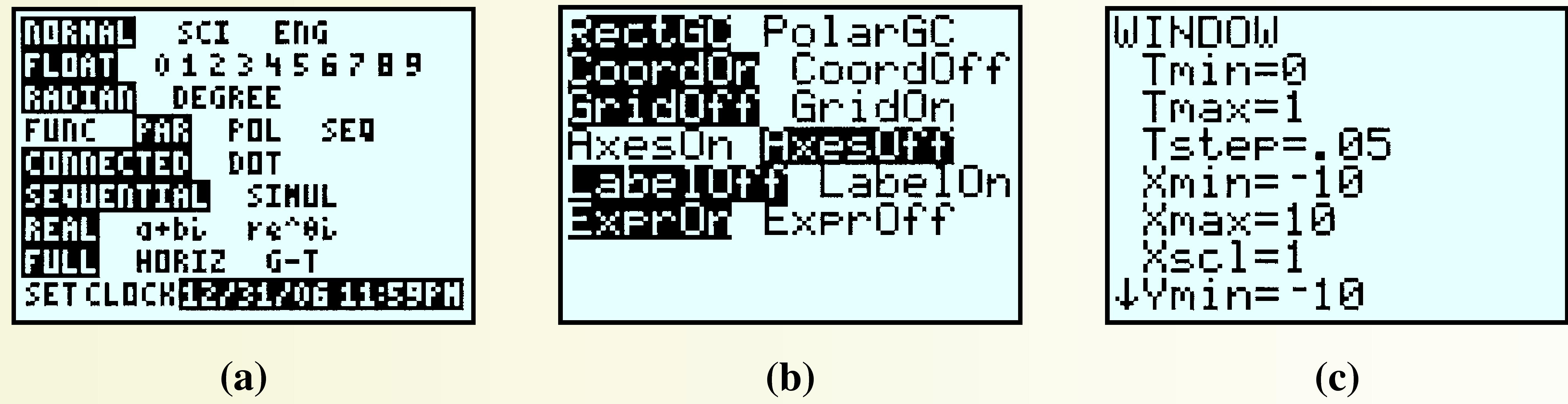
We can draw Bézier curves on the graphing calculator using the parametric mode. First, press the MODE key and highlight PAR, as shown in figure (a). To remove the \(x\)- and \(y\)-axes from the display, press 2nd ZOOM to get the \(Format\) menu, then choose \(AxesOff\) as shown in figure (b). Finally, we set the viewing window: Press WINDOW and set

\begin{equation*} \begin{aligned}[t] \text{Tmin} \amp = 0 \amp \text{Tmax} \amp= 1\amp\text{TStep} \amp= 0.05\\ \text{Xmin} \amp = -10 \amp \text{Xmax} \amp= 10 \amp \text{Ymin} \amp = -10 \amp \text{Ymax} \amp= 10 \end{aligned} \end{equation*}

as shown in figure (c).

As an example, we will graph the linear curve from part (A). Press Y= and enter the definitions for \(x(t)\) and \(y(t)\text{,}\) as shown below. Press GRAPH and the calculator displays the line segment joining \((-4, 7)\) and \((2, 0)\text{.}\) Experiment by modifying the endpoints to see how the graph changes.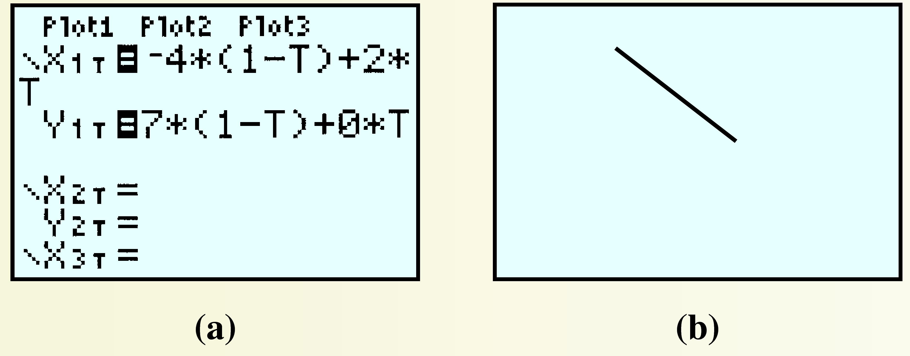
Designing a Numeral 7
1. Press 2nd Y= and enter the formulas for the quadratic Bézier curve defined by the endpoints \((4, 7)\) and \((0,-7)\text{,}\) and the control point \((0, 5)\) under \(X_{1T}\) and \(Y_{1T}\text{.}\) (These are the same formulas you found in step B.1 of Investigation 7.1.)
2. Find the functions \(f\) and \(g\) for the linear Bézier curve joining the points \((-4, 7)\) and \((4, 7)\text{.}\) Simplify the formulas for those functions and enter them into your calculator under \(X_{2T}\) and \(Y_{2T}\text{.}\) Press GRAPH to see the graph.
3. Now we will alter the image slightly: Go back to \(X_{1T}\) and \(Y_{1T}\) and change the control point to \((0,-3)\text{.}\) (These are the formulas you found in step B.4 of Investigation 7.1.) How does the graph change?
4. We can see exactly how the control point affects the graph by connecting the three data points with line segments. Press STAT ENTER and enter the coordinates of \((4, 7)\text{,}\) \((0,-3)\text{,}\) and \((0,-7)\) in \(L_1\) and \(L_2\text{,}\) as shown in figure (a). Press 2nd Y= ENTER, turn on Plot1, and select the second plot type, as shown in figure (b). You should see the line segments superimposed on your numeral 7. How are those segments related to the curve?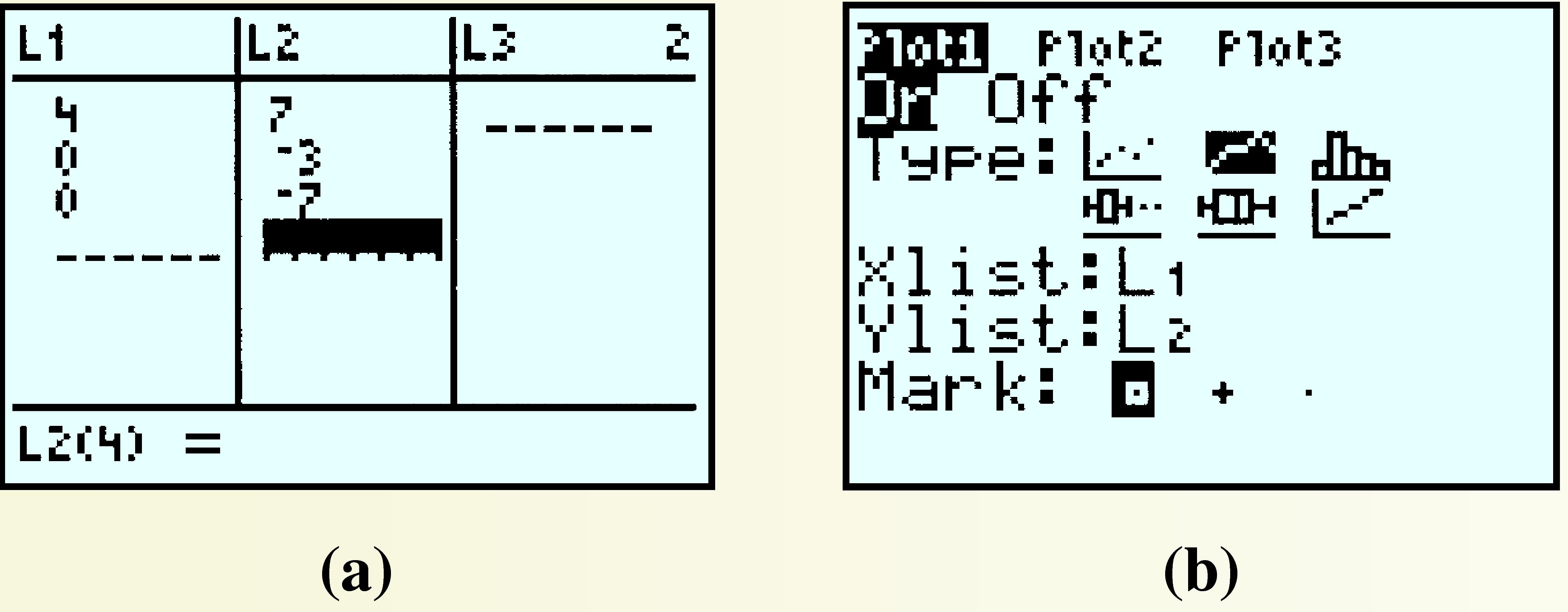
5. Now edit \(L_2\) so that the control point is \((0, 5)\text{,}\) and again define \(X_{1T}\) and \(Y_{1T}\) as in step B.1 to see how the graph is altered. Experiment by using different coordinates for the control point and entering the appropriate new equations in \(X_{1T}\) and \(Y_{1T}\text{.}\) Describe how the point \((x_2, y_2)\) affects the direction of the quadratic Bézier curve.
  Hint
  Consider the direction of the curve starting off from either endpoint.
Designing a Letter y with Cubic Bézier Curves
1. First, turn off Plot1 by pressing Y= \(\boxed{\uparrow}\) ENTER.
2. Enter the formulas for the cubic Bézier curve from part C.1 under \(X_{1T}\) and \(Y_{1T}\text{.}\) Modify the expressions in \(X_{2T}\) and \(Y_{2T}\) to the linear Bézier curve joining the points \((-4, 7)\) and \((2, 0)\) from step A.1 of Investigation 7.1.
3. How do the control points affect the direction of the Bézier curve? (Suggestion: Enter the coordinates of the four points under \(L_1\) and \(L_2\) and turn Plot1 back on.)

When you finish experimenting with Bézier curves, set the calculator MODE (2nd QUIT) back to FUNC, and reset the FORMAT(2nd ZOOM)to AxesOn.

Technology D.19. Solving Equations with Fractions Graphically.

We can solve the equation in Example 7.68 graphically by considering two functions, one for each side of the equation. Graph the two functions

\begin{equation*} Y_1=\frac{30}{12+x} \hphantom{space}\text{and}\hphantom{space}Y_2=\frac{30}{12-x} \end{equation*}

in the window

\begin{align*} \text{Xmin} \amp = -9.4 \amp\amp \text{Xmax} = 9.4\\ \text{Ymin} \amp = 0 \amp\amp \text{Ymax} = 10 \end{align*}

to obtain the graph shown below.

The function \(Y_1\) gives the time it takes Rani to paddle 30 miles downstream, and \(Y_2\) gives the time it takes her to paddle \(18\) miles upstream. Both of these times depend on the speed of the current, \(x\text{.}\)

We are looking for a value of \(x\) that makes \(Y_1\) and \(Y_2\) equal. This occurs at the intersection point of the two graphs, \((3, 2)\text{.}\) Thus, the speed of the current is \(3\) miles per hour, as we found in Example 7.68. The y-coordinate of the intersection point gives the time Rani paddled on each part of her trip: \(2\) hours each way.

Technology D.20. Using the Intersect Feature to Solve a System.

Because the TRACE feature does not show every point on a graph, we may not find the exact solution to a system by tracing the graphs. In the next Example we demonstrate the intersect feature of the calculator.

Example D.21.

Solve the system

\begin{align*} 3x - 2.8y \amp= 21.06\\ 2x + 1.2y \amp= 5.3 \end{align*}

Solution

We can graph this system in the standard window by solving each equation for \(y\text{.}\) We enter

\begin{align*} Y_1\amp = (21.06 - 3X)/-2.8\\ Y_2\amp = (5.3 - 2X)/1.2 \end{align*}

and then press ZOOM \(6\text{.}\) (Don't forget the parentheses around the numerator of each expression.)

We Trace along the first line to find the intersection point. It appears to be at \(x=4.468051\text{,}\) \(y =-2.734195\text{,}\) as shown in figure (a). However, if we press the up or down arrow to read the coordinates off the second line, we see that for the same \(x\)-coordinate we obtain a different \(y\)-coordinate, as in figure (b).

The different \(y\)-coordinates indicate that we have not found an intersection point, although we are close. The intersect feature can give us a better estimate, \(x = 4.36\text{,}\) \(y = -2.85\text{.}\)

GC display of 2 lines intersecting in 4th quadrant

We can substitute these values into the original system to check that they satisfy both equations.

\begin{align*} 3(\alert{4.36}) - 2.8(\blert{-2.85}) \amp = 21.06\\ 2(\alert{4.36}) + 1.2(\blert{-2.85}) \amp = 5.3 \end{align*}

Technology D.22.

TI-84 and TI-83 calculators have a command for finding the reduced row echelon form of a matrix.

Example D.23.

Solve the system

\begin{alignat*}{5} a\amp {}+{} \amp 2b \amp {}+{}\amp 4c\amp {}+{}\amp 8d \amp =\amp 12\\ -2a\amp {}+{}\amp 2b\amp {}-{}\amp 2c\amp {}+{}\amp 2d \amp =\amp 1\\ 6a\amp {}+{}\amp 6b\amp {}+{}\amp 6c\amp {}+{}\amp 6d\amp =\amp 19\\ 4a\amp {}+{}\amp 20b\amp {}-{}\amp 8c\amp {}+{}\amp 14d\amp =\amp 41 \end{alignat*}

by finding the reduced row echelon form of the augmented matrix.

Solution

The augmented matrix is

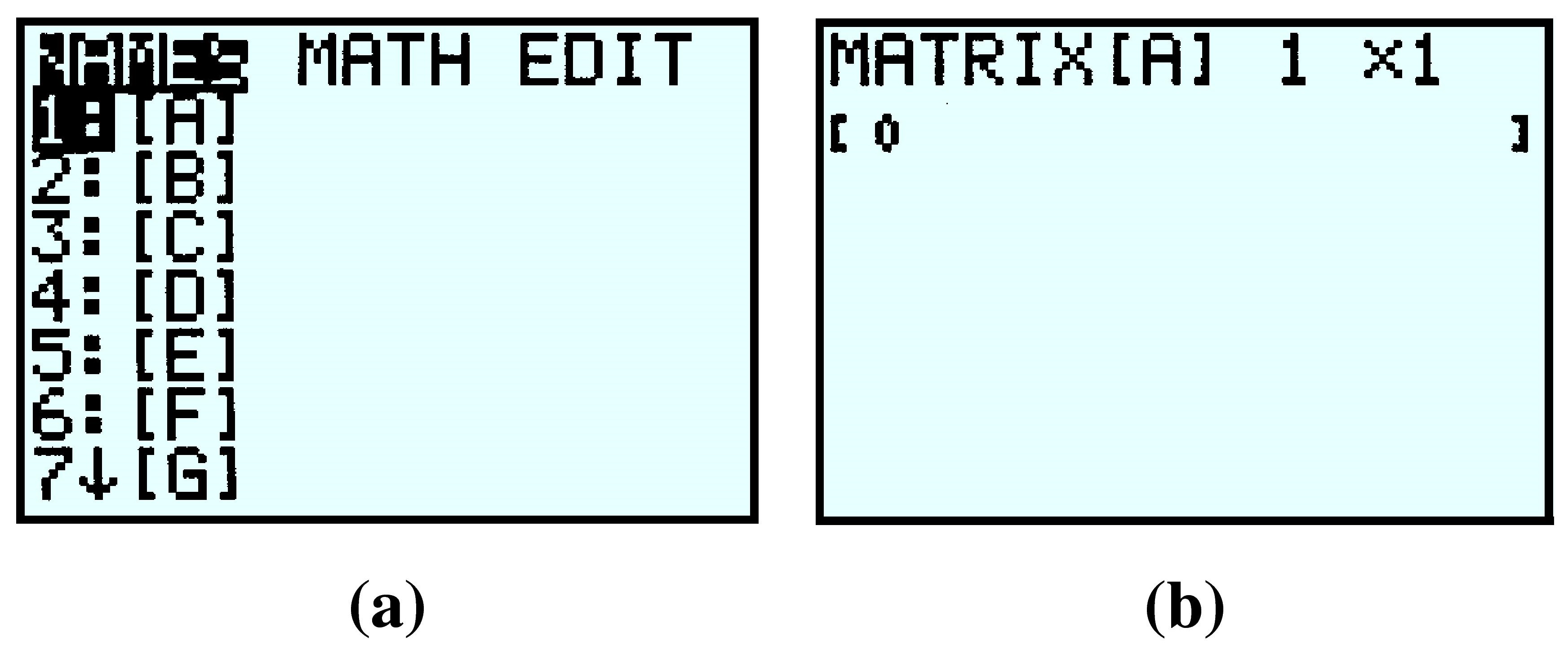
\begin{equation*} \left[ \begin{array}{@{}cccc|c@{}} 1 \amp 2 \amp 4 \amp 8 \amp 12 \\ -2\amp 2 \amp -2\amp 2 \amp 1 \\ 6 \amp 6 \amp 6 \amp 6 \amp 19 \\ 4 \amp 20 \amp -8\amp 14\amp 41 \end{array}\right] \end{equation*}

We enter this matrix into the calculator as follows: First access the MATRIX menu by pressing 2nd \(\boxed{x^{-1}}\) on a TI-84 orMATRX on a TI-83. You will see the menu shown in figure (a). We will use matrix [A], which is already selected, and we presss \(\boxed{\rightarrow}\) \(\boxed{\rightarrow}\) ENTER to EDIT (or enter) the matrix, shown in figure(b).

We want to enter a \(4\times 5\) matrix, so we press \(4\)ENTER\(5\)ENTER, and we see the display in figure (a) below. Now type in the first row of the matrix, pressing ENTER after each entry. The calculator automatically moves to the second row. Continue filling in the rest of the augmented matrix, as shown in figure (b).

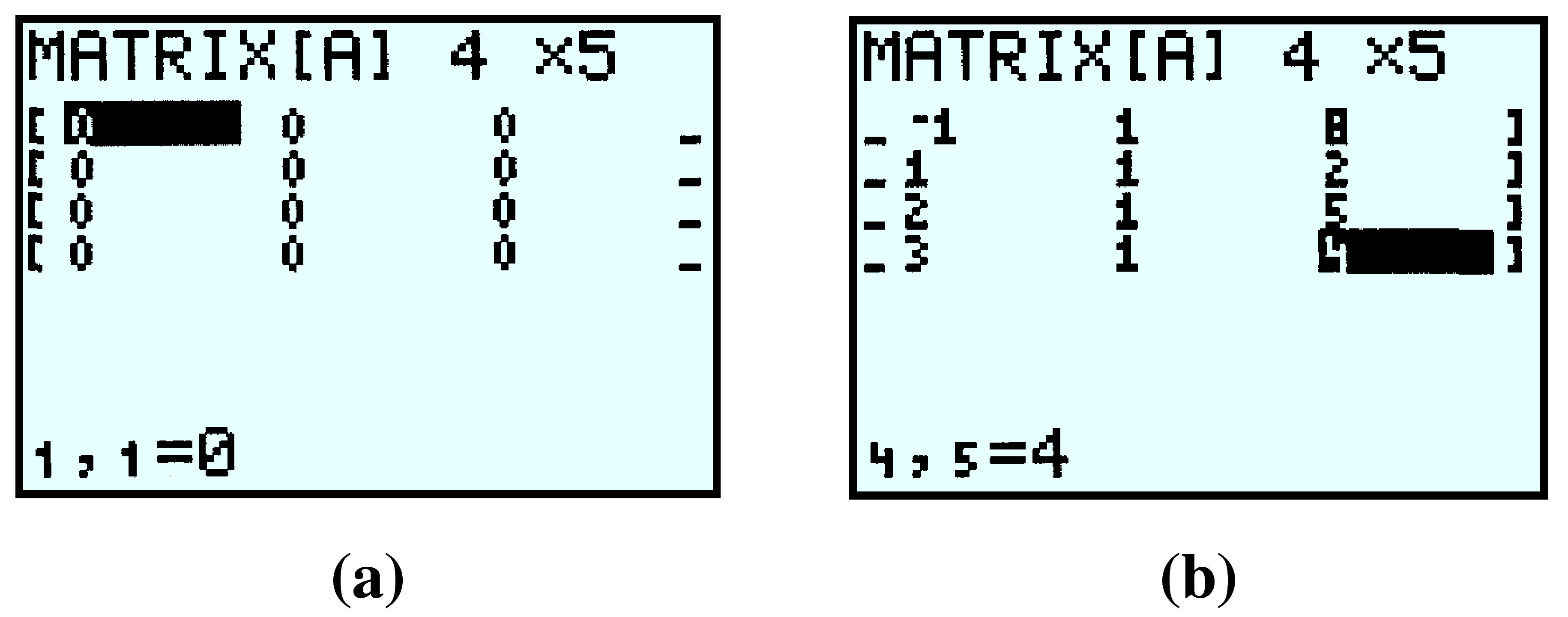
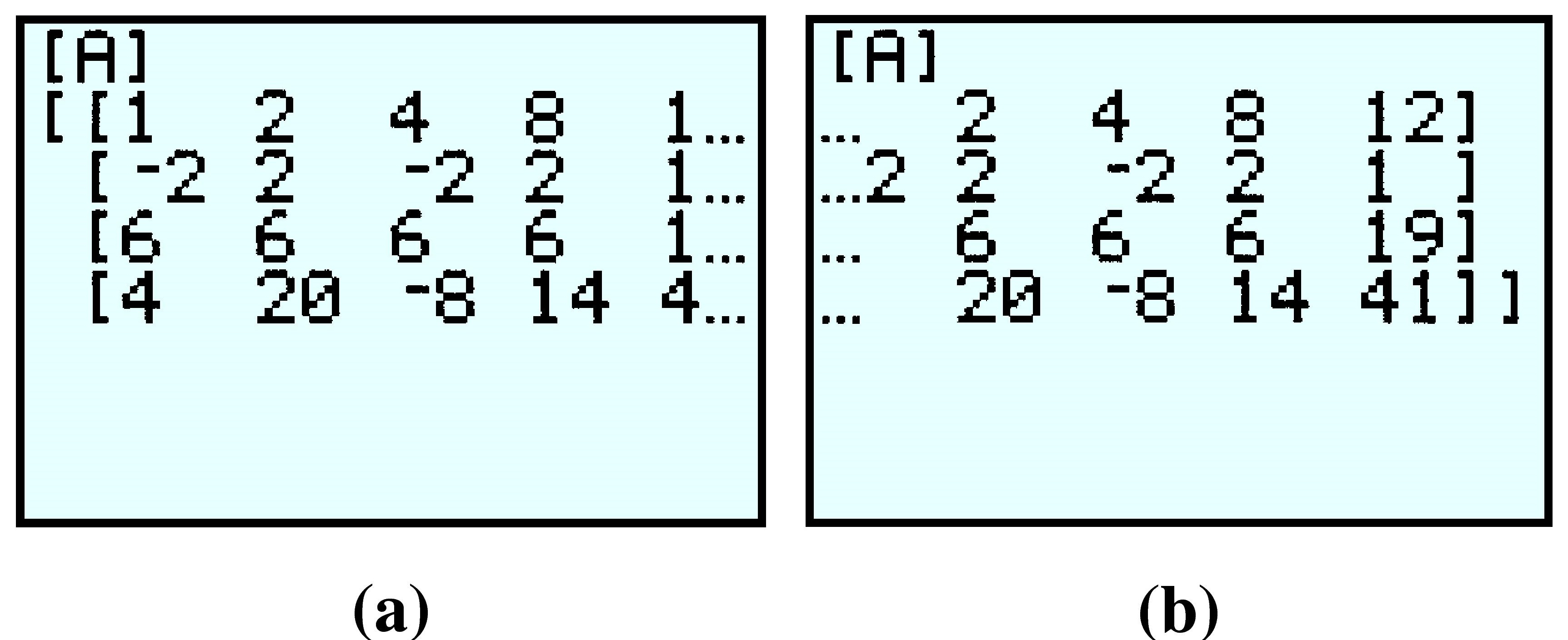
To make sure you have entered the values correctly, press 2ndMODE to quit to the home screen, then open the matrix menu again. Press \(1\)ENTER to retrieve matrix [A]; the calculator display should look like figure (a) below. To check the rest of the matrix, press the right arrow key until you see the last column, as in figure (b).

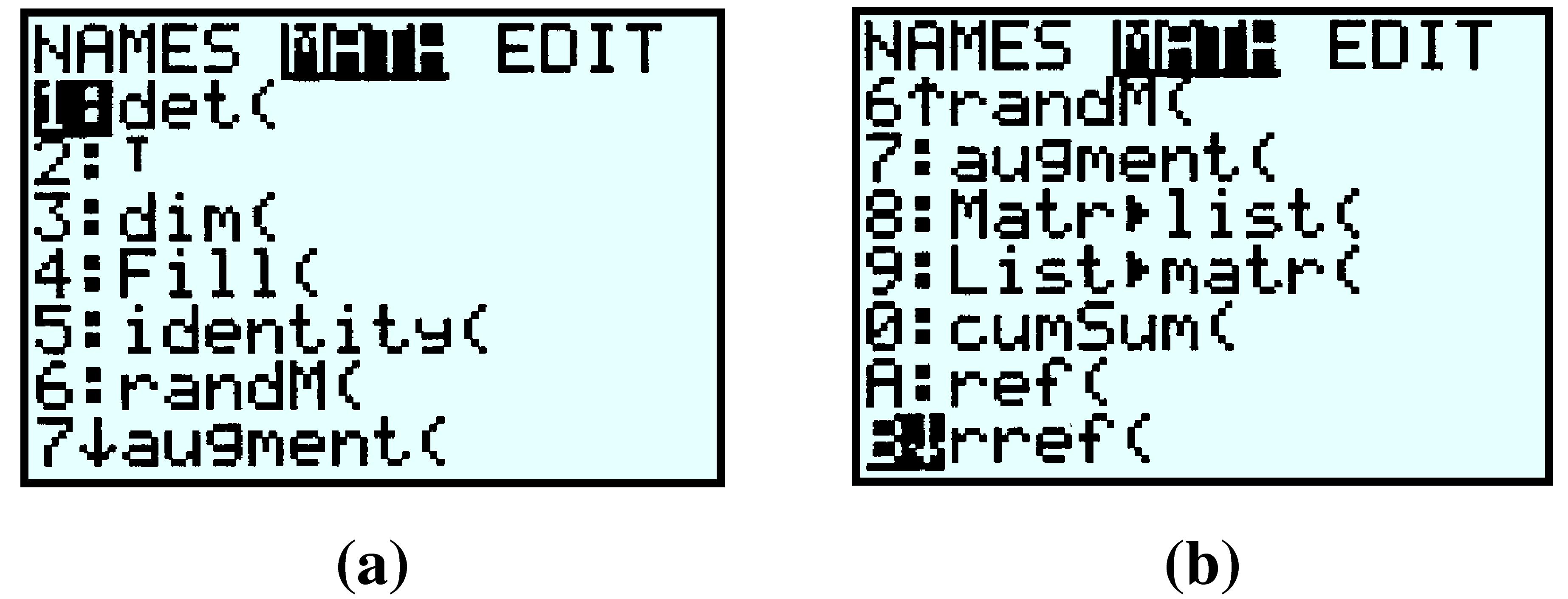
Now we are ready to compute the reduced row echelon form of the matrix. Access the matrix menu again, but this time press the right arrow once to highlight MATH as shown in figure (a). Scroll down until the rref( command is highlighted, as shown in figure (b), and press ENTER.

Finally, enter matrix [A] after the rref( command by pressing 2nd \(\boxed{x^{-1}}\) \(1\)) ENTER or \(MATRX\) \(1\)) ENTER. The display should now look like figure (a) below. The last column of the matrix gives decimal approximations for the solutions.

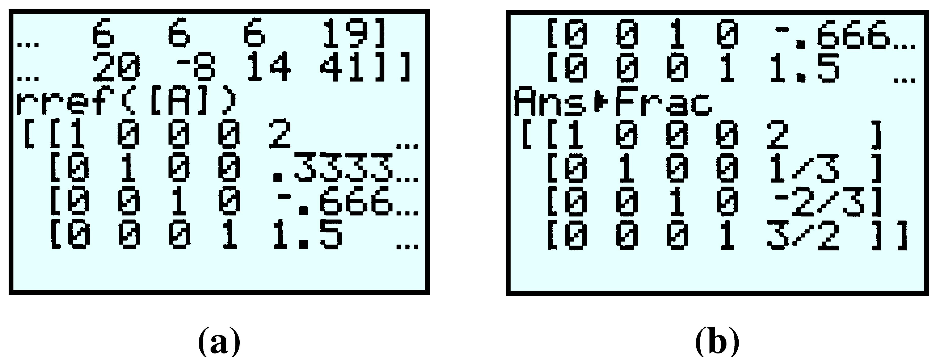
The calculator can also display the rational form of the solutions: Press MATH ENTER ENTER to see figure(b). The reduced row echelon form of the augmented matrix is thus

\begin{equation*} \left[ \begin{array}{@{}cccc|c@{}} 1 \amp 0 \amp 0 \amp 0 \amp 2 \\ 0 \amp 1 \amp 0 \amp 0 \amp 1/3 \\ 0 \amp 0 \amp 1 \amp 0 \amp -2/3 \\ 0 \amp 0 \amp 0 \amp 1 \amp 3/2 \end{array}\right] \end{equation*}

and the solution is the ordered four-tuple \((2, \dfrac{1}{3}, \dfrac{-2}{3}, \dfrac{3}{2})\text{.}\) You can verify that these values satisfy each of the original four equations.